Rice Classification

This example of Matlab attempts to show how can we do Image Analysis by segmenting and classifying objects in an image.

This program counts the number of rice present in an image. In addition, the average and standard deviation of the size are computed.

WARNING: the presented solution is very simple. The goal of this code is to show how can we use Matlab in Image Analysis. Obviously, better results can be obtained using more complex algorithms.

Computer Vision Course

1. Image acquisition
2. Image display
3. Histogram
4. Segmentation using a global threshold
5. Background elimination
6. Segmentation of the new image
7. Elimination of small regions (isolated pixeles)
8. Labeling of regions
9. Feature extraction
10. Classification of regions
11. Results

1. Image acquisition

In this part, we read a digital gray-scale image, and we store it in a matrix using two formats:

a) 'uint8' for bytes (uint8: unsigned integer with 8 bits) and

b) 'double' for double precision.

close all                    % All figures are closed
clear all                    % All variables are deleted
U = imread('rice.png');      % Read image rice.png
I = double(U);               % Conversion to double

2. Image display

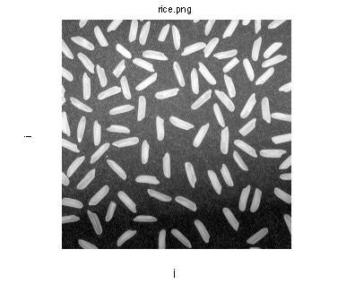
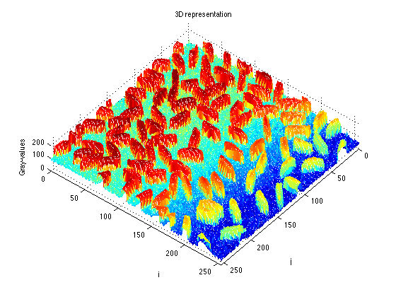
In this part, we display the image using grayscale and 3D representations. In addition, we label the axes.

figure                       % Open new figure
imshow(I,[])                 % Display image I: min(I) is black max(I) is white
title('rice.png')            % Title of the figure
xlabel('j');                 % Name of the x-axis
ylabel('i');                 % Name of the y-axis

figure                       % Open new figure
mesh(I)                      % 3D mesh surface
view(129,78)                 % view point
title('3D representation')   % Title of the figure
xlabel('j');                 % Name of x-axis
ylabel('i');                 % Name of y-axis
zlabel('Gray-values');       % Name of z-axis
axis([0 255 0 255 0 255]);   % Range of x,y,z in 3D representation

3. Histogram

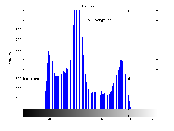
In this part, we compute the histogram of the image, i.e., how many pixels we have in the image for each gray-value.

figure                       % Open new figure
imhist(U)                    % Histogram of uint8 image
title('Histogram')           % Title of the figure
xlabel('Gray-values');       % Name of x-axis
ylabel('Frequency');         % Name of y-axis
text(1,300,'background')
text(200,300,'rice')
text(120,900,'rice & background')

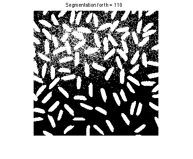
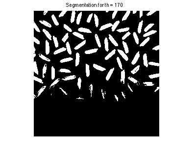
4. Segmentation using a global threshold

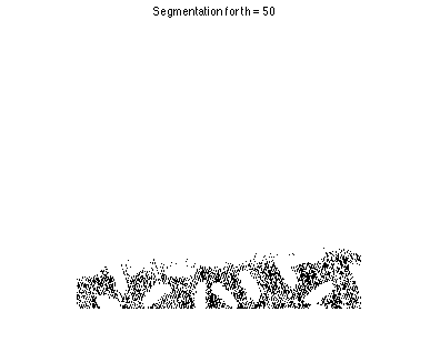
In this part, we compute a binary image B by thresholding.

In this case, B(i,j) = 1 if I(i,j)>th, else B(i,j) = 0. Ideally, B(i,j) = 1 if the pixel (i,j) belongs to the rice region, and it is 0 if it belongs to the background.

However, a global threshold does not segment well the image because the certain gray-values of the background (top of the image) are similar to certain gray-avlues of the rice (bottom of the image).

for th = 50:60:170           % th takes 50, 50+60=110 and 170
    figure
    B = I>th;                % Binary image: '1' for gray-values>th
    imshow(B)
    s = sprintf('Segmentation for th = %d',th);
    title(s);
end

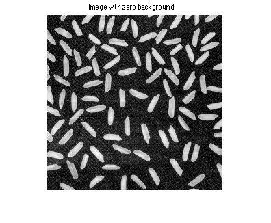
5. Background elimination

Since the background is not homogoneous (the top is brighter than the bottom), in this part, we attemp to set the background to zero. Thus, each row will be updated by subtracting its minimal value.

[N,M] = size(I);
J     = zeros(N,M);

for i=1:N
    row_i  = I(i,:);         % vector that contains the i-th row of I
    mi     = min(row_i);     % minimal value of i-th row
    J(i,:) = row_i-mi;       % each row is decreased by its minimum
end

figure
imshow(J,[])
title('Image with zero background')

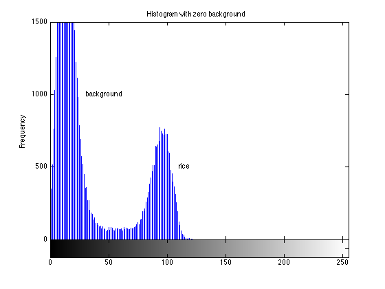
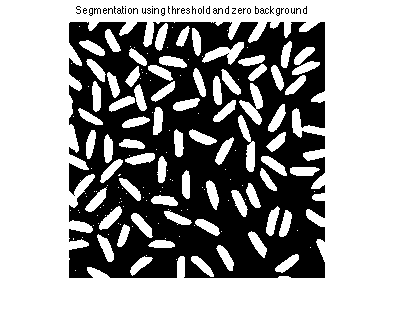
6. Segmentation of the new image

In this part, we segment the new image (with zero background) using a global threshold. First, we display the histogram where background and forground are clearly distinguishable. Second, we display the new binary image using a threshold = 40.

figure
imhist(uint8(fix(J)))
title('Histogram with zero background')
xlabel('Gray-values');
ylabel('Frequency');
text(30,1000,'background')
text(110,500,'rice')

figure
K = J>40;                    % pixels which gray-values are greater than 40 are segmented
imshow(K)
title('Segmentation using threshold and zero background');

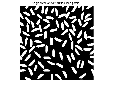
7. Elimination of small regions (isolated pixeles)

We observe that the new segmentation image has isolated pixels. They correspond to noise in the background. In this part, we eliminate those pixles using command 'bwareaopen'.

T = bwareaopen(K,20);        % regions which size is less than 20 pixels are eliminated
figure
imshow(T)
title('Segmentacion without isolated pixels')

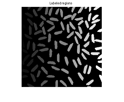
8. Labeling of regions

In order to perform a pattern recognition approach (with feature extraction and classification), we label each isolated region using the command 'bwlabel'.

L = bwlabel(T);              % We assign a label to each region
n = max(L(:));               % Number of regions
figure
imshow(L,[])                 % Each region has a different gray-value
title('Labeled regions')
hold on

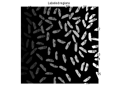
9. Feature extraction

In this part, for each labeled region we compute the size (area in pixels) and the center of mass (x,y in pixels). The area will be used in the classification. The location (x,y) will not be used in the classification, it will be used only for printing the label number of each rice.

A = zeros(n,1);              % Area
x = zeros(n,1);              % Location x
y = zeros(n,1);              % Location y

for i=1:n
    R = L==i;               % Binary image '1' means pixel belongs to region i
    [ii,jj] = find(R==1);   % Coordinates of each pixel of region i
    A(i) = length(ii);      % Area of region i
    x(i) = mean(jj);        % x value of center of mass of region i
    y(i) = mean(ii);        % y value of center of mass of region j
    text(x(i),y(i),num2str(i))
end

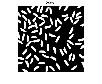
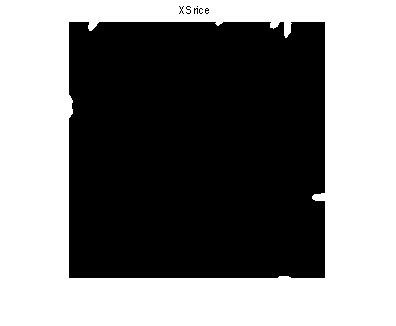
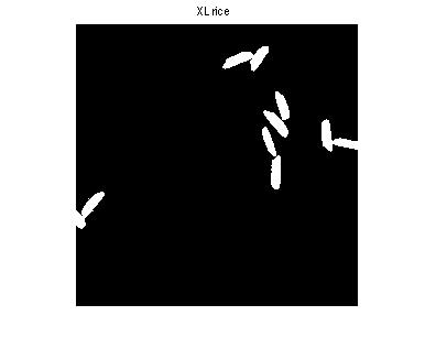
10. Classification of regions

In this part, we attempt to classify each region in one of three classes: XS (extra-small), OK and XL (extra-large). XS regions correspond to regions that are incomplete (e.g. region 95). XL regions correspond to regions that are joined (e.g. region 55).

IXS = zeros(N,M);            % Image with XS rice
IXL = zeros(N,M);            % Image with XL rice
IOK = zeros(N,M);            % Image with OK rice
t   = 0;                     % count of segmented regions
AOK = zeros(n,1);            % area of segmented regions
for i=1:n
    R = L==i;                % We look for region i
    a = A(i);                % Area of region i
    if (a<100)               % XS regions
        IXS = or(IXS,R);     % Adding XS regions
    else
        if (a>300) % XL regions
            IXL = or(IXL,R); % Adding XL regions
        else
            IOK = or(IOK,R); % Adding OK regions
            t = t + 1;
            AOK(t) = a;
        end
    end
end

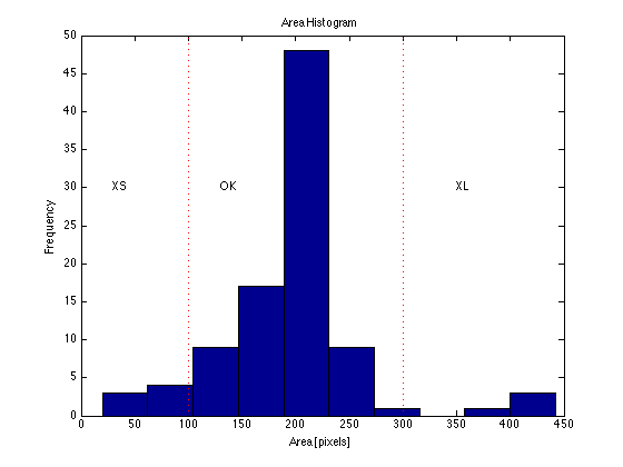
11. Results

In this part we display the results. One image for each class. In addition, we display the histogram of area, and average size and standard deviation.

figure
imshow(IOK)
title('OK rice');

figure
imshow(IXS)
title('XS rice');

figure
imshow(IXL)
title('XL rice');

figure
hist(A)
hold on
plot([100 100],[0 50],'r:')
plot([300 300],[0 50],'r:')
title('Area Histogram');
xlabel('Area [pixels]');
ylabel('Frequency');
text(30 ,30,'XS');
text(130,30,'OK');
text(350,30,'XL')


p = mean(AOK(1:t));   % mean of the segmented regions
s = std(AOK(1:t));    % standard deviation of segmented regions
disp('Statistics of OK rice:')
fprintf('    >               Count: %d\n',t)
fprintf('    >        Average area: %6.2f [pixels]\n',p)
fprintf('    >  Standard deviation: %6.2f [pixels]\n',s)

Statistics of OK rice:
    >               Count: 83
    >        Average area: 195.34 [pixels]
    >  Standard deviation:  32.78 [pixels]